Apply analytical methods

The replicator dynamics

The replicator equation represents the dynamics of competing individuals in an infinite population (\(Z\rightarrow \infty\)). It defines the rate at which the frequency of strategies in a population will change, i.e., it defines a gradient of selection [2]. It is often found in the form of [4]

\[\dot x_{i} = x_{i} \left(f_i(\vec{x})-\sum_{j=1}^{N}{x_{j}f_j(\vec{x})}\right)\]

where \(x_i\) represents the frequency of strategy \(i\) in the population, and \(f_i(\vec{x})=\Pi_i(\vec{x})\) its fitness (or expected payoff), given the current population state \(\vec{x}\). The term \(\sum_{j=1}^{N}{x_{j}f_j(\vec{x})}\) represents the average fitness of the population in state \(\vec{x}\).

EGTtools implements the replicator equation for 2 and N-player games in the functions egttools.analytical.replicator_equation and egttools.analytical.replicator_equation_n_player. Both methods require a payoff matrix as argument. For 2-player games, this payoff matrix must be square and have as many rows (columns) as strategies in the population. For N-player games, the payoff_matrix reads as the payoff of the row strategy at the group configuration given by the index of the column. The group configuration can be retrieved from the index using egttools.sample_simplex(index, group_size, nb_strategies), where group_size is the size of the group (N) and nb_strategies is the number of available strategies in the population.

2-player games

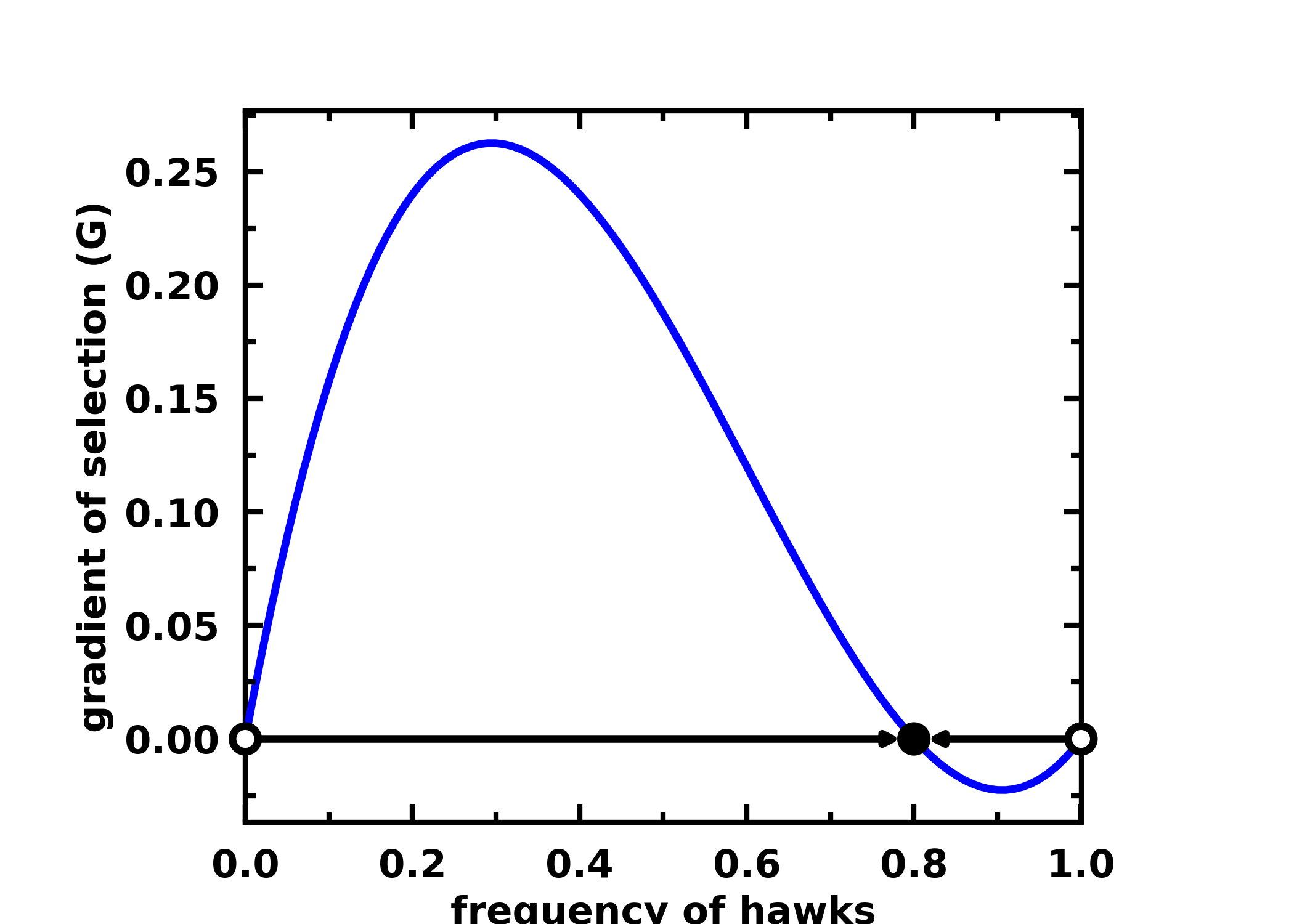
For a 2 player hawk-dove game, you can calculate the gradients of selection, the roots and their stability with:

import numpy as np
import egttools as egt
from egttools.analytical.utils import (calculate_gradients, find_roots, check_replicator_stability_pairwise_games, )

# Calculate gradient
payoffs = np.array([[-0.5, 2.], [0., 0]])
x = np.linspace(0, 1, num=101, dtype=np.float64)
gradient_function = lambda x: egt.analytical.replicator_equation(x, payoffs)
gradients = calculate_gradients(np.array((x, 1 - x)).T, gradient_function)

# Find roots and stability
roots = find_roots(gradient_function, nb_strategies=2, nb_initial_random_points=10, method="hybr")
stability = check_replicator_stability_pairwise_games(roots, A)

# Plot the gradient
egt.plotting.plot_gradients(gradients[:, 0], xlabel="frequency of hawks", roots=roots, stability=stability)

You can then plot the gradient of selection with:

egt.plotting.plot_gradients(gradients[:, 0], xlabel="frequency of hawks", roots=roots, stability=stability)

You can find other examples here.

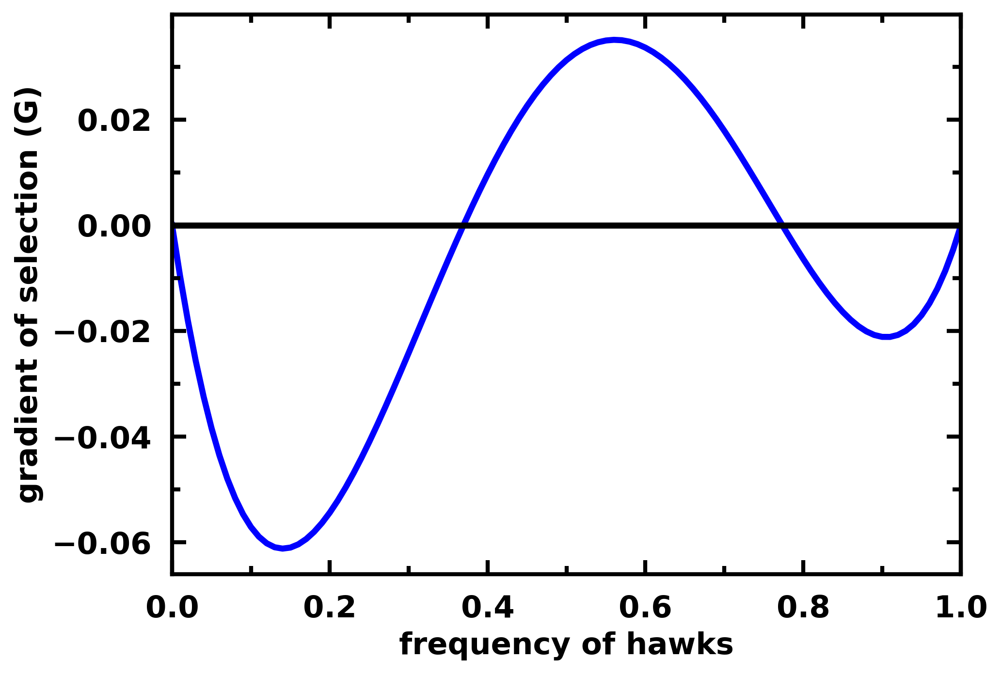
N-player games

When \(N>2\), the game is played among groups of more than 2 players. In this case, to analyse the replicator dynamics, we need to use egt.analytical.replicator_equation_n_player instead.

For example for a 3-player Hawk-Dove game we have:

payoff_matrix = np.array([
    [-0.5,  2. ,  1. ,  3. ],
    [ 0. ,  0. ,  1. ,  2. ]
])

gradient_function = lambda x: egt.analytical.replicator_equation_n_player(x, payoff_matrix, group_size=3)
gradients = calculate_gradients(np.array((x, 1 - x)).T, gradient_function)

# Plot the gradient
egt.plotting.plot_gradients(gradients[:, 0], xlabel="frequency of hawks")

Note

For the moment egttools only supports the analytical calculation of stability for the replicator equation for 2-player games. We have planned to add support for N-player games in version 0.13.0.

Stochastic dynamics in finite populations: the pairwise comparison rule

The replicator dynamics assumes that populations have infinite size. This is convenient from a technical point of view, as it allows using relatively simple differential equations to model complex evolutionary processes. However, in many occasions, when modelling realistic problems, we cannot neglect the stochastic effects that come along when individuals interact in finite populations [5].

We now consider a finite population of \(Z\) individuals, who interact in groups of size \(N\in[2,Z]\), in which they engage in strategic interactions (or games). Each individual can adopt one of the \(n_s\) strategies. The success (or fitness) of an individual can be computed as the expected payoff of the game in a given state \(\vec{x}\).

We adopt a stochastic birth-death process combined with the pairwise comparison rule [1, 5, 6] to describe the social learning dynamics of each of the strategies in a finite population. At each time-step, a randomly chosen individual \(j\) adopting strategy \(\vec{e_{j}}\) has the opportunity to revise her strategy by imitating (or not) the strategy of a randomly selected member of the population \(i\). The imitation will occur with a probability \(p\) which increases with the fitness difference between \(j\) and \(i\). Here we adopt the Fermi function (see Equation below), which originates from statistical physics and provides a well defined mapping between \(\mathbb{R}^+ \rightarrow [0,1]\). Please also note that since the population is finite, instead of assuming the frequencies of each strategy in the population (\(x_i\)) we use the absolute value \(k_i\) so that \(x_i \equiv[k_i/Z]\).

\[\begin{equation} \label{eq:fermi_function} p\equiv[1+e^{\beta(f_i(k_{i})-f_j(k_{j}))}]^{-1} \end{equation}\]

In equation above, \(f_j\) (\(f_i\)) is the fitness of individual \(j\) (\(i\)) and \(\beta\), also known as inverse temperature, controls the intensity of selection and the accuracy of the imitation process. For \(\beta \rightarrow 0\), individual fitness is but a small perturbation to random drift; for \(\beta \rightarrow\infty\) imitation becomes increasingly deterministic. Also, \(k_{i}\) represents again the total number of individuals adopting strategy \(i\). In addition, we consider that, with a mutation (or exploration) probability \(\mu\), individuals adopt a randomly chosen strategy, freely exploring the strategy space. Overall this adaptive process defines a large-scale Markov chain, in which the transition probabilities between states are defined in function of the fitness of the strategies in the population and their frequency. The complete characterization of this process becomes unfeasible as the number of possible population configurations scales with the population size and the number of strategies following \(\binom{Z+n_s-1}{n_s-1}\) [7].

The probability that the number \(k\) of participants adopting a cooperative strategy \(C\) would increase (\(T^+(k)\)) or decrease (\(T^-(k)\)) can be specified as [5]:

\[\begin{split}\begin{equation} \label{eq:prob_increase_decrease} \begin{split} T^+ &= (1-\mu)\frac{Z-k}{Z}\frac{k}{Z-1}[1+e^{-\beta(f_i-f_j)}]^{-1} + \mu\frac{Z-k}{Z}\\ T^- &= (1-\mu)\frac{k}{Z}\frac{Z-k}{Z-1}[1+e^{\beta(f_i-f_j)}]^{-1} + \mu\frac{k}{Z}\\ \end{split} \end{equation}\end{split}\]

Small Mutation Limit (SML)

The Markov chain described above can quickly become too complex for analytical description as the number of strategies, even for small population sizes. However, whenever in the limit where mutations are rare (\(\mu \rightarrow 0\)) it is possible to approximate the complete stochastic process by a Markov chain with a number of states given by the number of strategies. In this small mutation limit (SML) [6], when a new strategy appears through mutation, one of two outcomes occurs long before the occurrence of a new mutation: either the population faces the fixation of a newly introduced strategy, or the mutant strategy goes extinct.

Hence, there will be a maximum of two strategies present simultaneously in the population. This allows us to describe the behavioural dynamics in terms of a reduced Markov Chain of size \(n_s\), whose transitions are defined by the fixation probabilities \(\rho_{ji}\) of a single mutant with strategy \(i\) in a population of individuals adopting another strategy \(j\) [5, 8, 9].

\[\begin{equation} \rho_{ji}=\left(1+\sum_{m=1}^{Z-1}\prod_{k=1}^m\frac{T^- (k)}{T^+ (k)}\right)^{-1} \end{equation}\]

How to use this model in EGTtools

All of these analytical equations are implemented in the class egttools.analytical.PairwiseComparison, which contains the following methods:

• calculate_fixation_probability(invading_strategy_index, resident_strategy_index:, beta:):

  Calculates the fixation probability of a single mutant of an invading strategy of index invading_strategy_index in a population where all individuals adopt the strategy with index resident_strategy_index. The parameter beta gives the intensity of selection.

• calculate_transition_and_fixation_matrix_sml(beta):

  Calculates the transition and fixation matrices assuming the SML. Beta gives the intensity of selection.

• calculate_gradient_of_selection(beta, state):

  Calculates the gradient of selection (without considering mutation) at a given population state. The state parameter must be an array of shape (nb_strategies,), which gives the count of individuals in the population adopting each strategy. This method returns an array indicating the gradient in each direction. In this stochastic model, gradient of selection means the most likely path of evolution of the population.

• calculate_transition_matrix(beta, mu):

  Calculates the transition matrix of the Markov chain that defines the dynamics of the population. beta gives the intensity of selection and mu the mutation rate.

You can see an example of the SML here, and of the calculation of the full transition matrix here.

Note

Currently, egttools only implements the moran process with the pairwise comparison rule. However, we have planned to add other evolutionary game theoretical models soon, such as the frequency dependant moran process or the Wright-Fisher process.

Note

We will add support for multiple populations soon.