Plot the evolutionary dynamics in a 2-Simplex
[1]:
import numpy as np
import matplotlib.pyplot as plt

%matplotlib inline
[2]:
import egttools as egt
[3]:
from egttools.plotting.helpers import (xy_to_barycentric_coordinates,
                                       barycentric_to_xy_coordinates,
                                       find_roots_in_discrete_barycentric_coordinates,
                                       calculate_stability,
                                    )
from egttools.analytical.utils import (find_roots, check_replicator_stability_pairwise_games, )
from egttools.helpers.vectorized import vectorized_replicator_equation, vectorized_barycentric_to_xy_coordinates
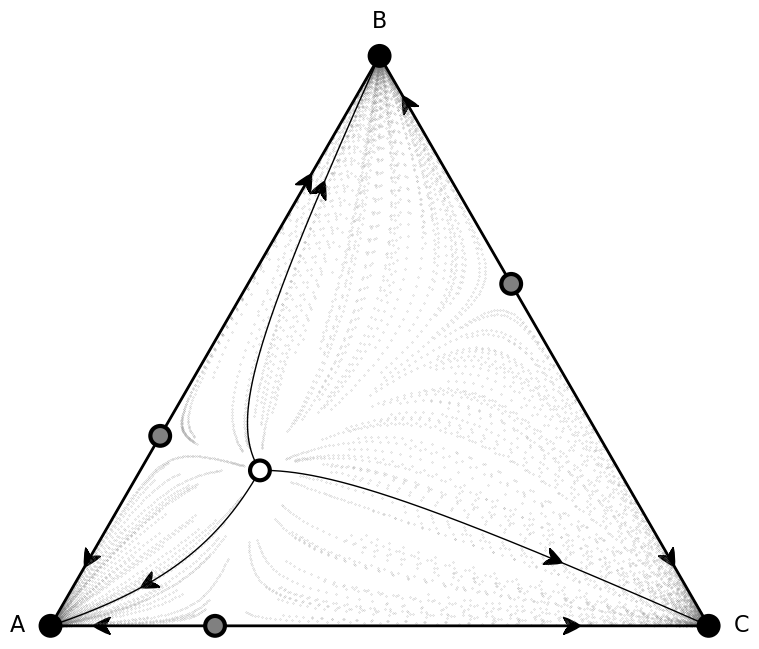
Evolutionary dynamics in infinite populations
In infinite populations the dynamics are given by the replicator equation. Following we calculate the gradients for all the points in a grid and plot them in a 2-simplex using the Simplex2D class.
We will also be plotting in the simplex the stationary points. We will use black circle to represent stable equilibrium and white circles to represent unstable ones. The arrows indicate the direction of the selective pressure.
Calculate gradients
[4]:
payoffs = np.array([[1, 0, 0],
                    [0, 2, 0],
                    [0, 0, 3]])
[5]:
simplex = egt.plotting.Simplex2D()
[6]:
v = np.asarray(xy_to_barycentric_coordinates(simplex.X, simplex.Y, simplex.corners))
[7]:
results = vectorized_replicator_equation(v, payoffs)
xy_results = vectorized_barycentric_to_xy_coordinates(results, simplex.corners)
Ux = xy_results[:, :, 0].astype(np.float64)
Uy = xy_results[:, :, 1].astype(np.float64)
[8]:
calculate_gradients = lambda u: egt.analytical.replicator_equation(u, payoffs)

roots = find_roots(gradient_function=calculate_gradients,
                   nb_strategies=payoffs.shape[0],
                   nb_initial_random_points=100)
roots_xy = [barycentric_to_xy_coordinates(root, corners=simplex.corners) for root in roots]

stability = check_replicator_stability_pairwise_games(roots, payoffs)
[9]:
type_labels = ['A', 'B', 'C']
[10]:
fig, ax = plt.subplots(figsize=(10,8))

plot = (simplex.add_axis(ax=ax)
           .apply_simplex_boundaries_to_gradients(Ux, Uy)
           .draw_triangle()
           .draw_stationary_points(roots_xy, stability)
           .add_vertex_labels(type_labels)
           .draw_trajectory_from_roots(lambda u, t: egt.analytical.replicator_equation(u, payoffs),
                                       roots,
                                       stability,
                                       trajectory_length=15,
                                       linewidth=1,
                                       step=0.01,
                                       color='k', draw_arrow=True, arrowdirection='right', arrowsize=30, zorder=4, arrowstyle='fancy')
           .draw_scatter_shadow(lambda u, t: egt.analytical.replicator_equation(u, payoffs), 300, color='gray', marker='.', s=0.1)
          )

ax.axis('off')
ax.set_aspect('equal')

plt.xlim((-.05,1.05))
plt.ylim((-.02, simplex.top_corner + 0.05))
plt.show()
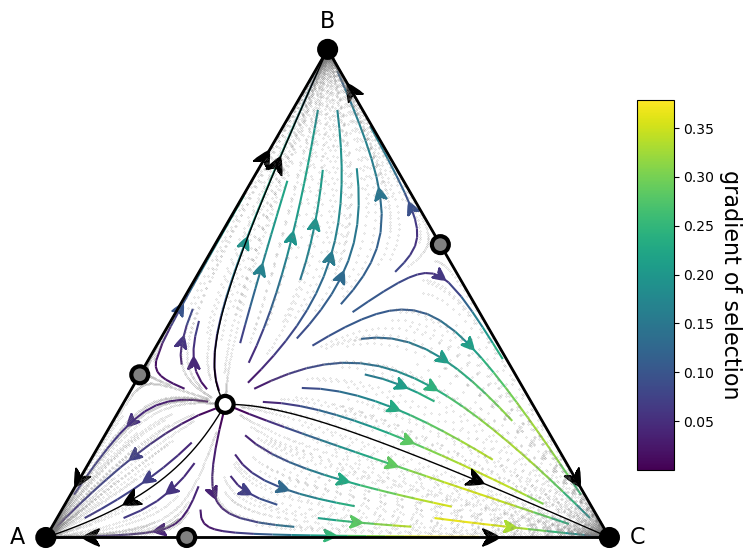
[11]:
fig, ax = plt.subplots(figsize=(10,8))

plot = (simplex.add_axis(ax=ax)
           .apply_simplex_boundaries_to_gradients(Ux, Uy)
           .draw_triangle()
           .draw_gradients(zorder=0)
           .add_colorbar()
           .draw_stationary_points(roots_xy, stability)
           .add_vertex_labels(type_labels)
           .draw_trajectory_from_roots(lambda u, t: egt.analytical.replicator_equation(u, payoffs),
                                       roots,
                                       stability,
                                       trajectory_length=15,
                                       linewidth=1,
                                       step=0.01,
                                       color='k', draw_arrow=True, arrowdirection='right', arrowsize=30, zorder=4, arrowstyle='fancy')
           .draw_scatter_shadow(lambda u, t: egt.analytical.replicator_equation(u, payoffs), 300, color='gray', marker='.', s=0.1, zorder=0)
          )

ax.axis('off')
ax.set_aspect('equal')

plt.xlim((-.05, 1.05))
plt.ylim((-.02, simplex.top_corner + 0.05))
plt.show()
Finite populations
In finite populations we will model the dynamics using a Moran process. The calculation of the gradients is implemented in EGTtools in the StochDynamics class. In this case, since we want to calculate the gradient at any point in the simplex, we will use the full_gradient_selection method
Calculate gradients
[12]:
Z = 100
beta = 1
mu = 1e-3
[13]:
simplex = egt.plotting.Simplex2D(discrete=True, size=Z, nb_points=Z+1)
[14]:
v = np.asarray(xy_to_barycentric_coordinates(simplex.X, simplex.Y, simplex.corners))
[15]:
v_int = np.floor(v * Z).astype(np.int64)
[16]:
evolver = egt.analytical.StochDynamics(3, payoffs, Z)
<ipython-input-16-ffdd52efb7d6>:1: DeprecationWarning: This class will soon be deprecated in favour of egttools.analytical.PairwiseComparison, which is implemented in c++ and runs faster, as well as, avoids precision issues that appeared in some limit cases.
  evolver = egt.analytical.StochDynamics(3, payoffs, Z)
[17]:
result = np.asarray([[evolver.full_gradient_selection(v_int[:, i, j], beta) for j in range(v_int.shape[2])] for i in range(v_int.shape[1])]).swapaxes(0, 1).swapaxes(0, 2)
[18]:
xy_results = vectorized_barycentric_to_xy_coordinates(result, simplex.corners)

Ux = xy_results[:, :, 0].astype(np.float64)
Uy = xy_results[:, :, 1].astype(np.float64)
[19]:
calculate_gradients = lambda u: Z*evolver.full_gradient_selection(u, beta)

roots = find_roots_in_discrete_barycentric_coordinates(calculate_gradients, Z, nb_interior_points=5151, atol=1e-1)
roots_xy = [barycentric_to_xy_coordinates(x, simplex.corners) for x in roots]

stability = calculate_stability(roots, calculate_gradients)
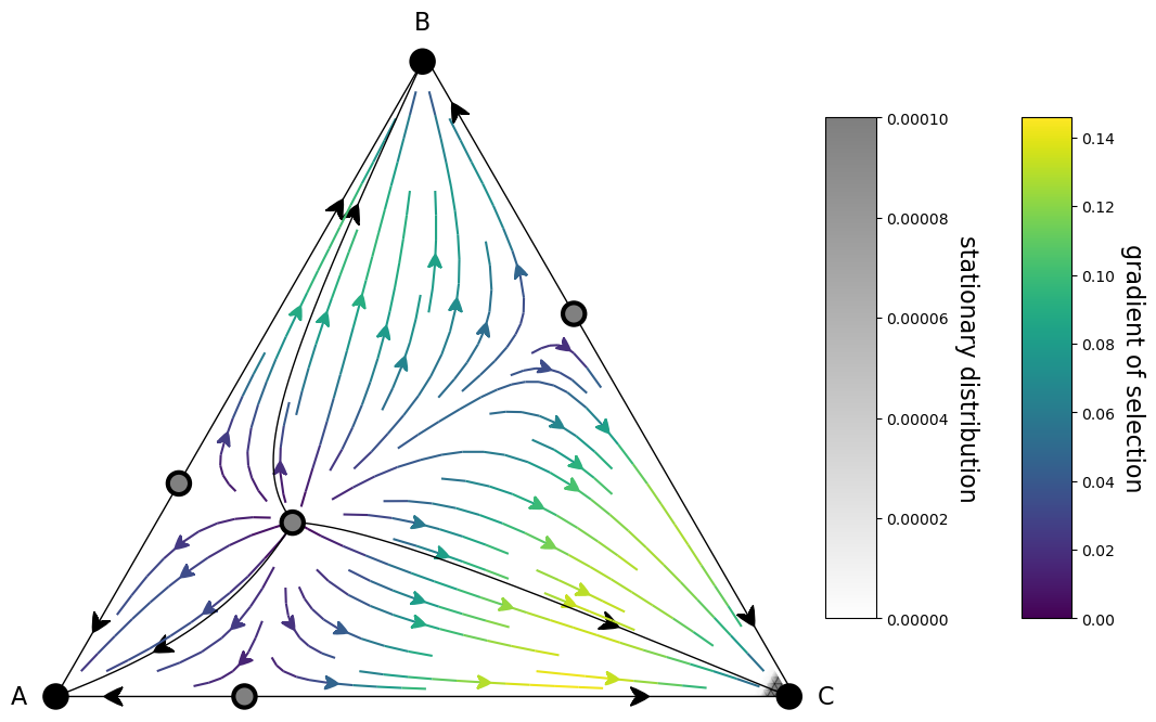
Calculate stationary distribution
We can also plot the stationary distribution inside the simplex. It will give us an idea on where our population is going to spend most of the time
[20]:
evolver.mu = 1e-3
sd = evolver.calculate_stationary_distribution(beta)
[21]:
fig, ax = plt.subplots(figsize=(15,10))

plot = (simplex.add_axis(ax=ax)
           .apply_simplex_boundaries_to_gradients(Ux, Uy)
           .draw_gradients(zorder=5)
           .add_colorbar()
           .draw_stationary_points(roots_xy, stability, zorder=11)
           .add_vertex_labels(type_labels)
           .draw_stationary_distribution(sd, vmax=0.0001, alpha=0.5, edgecolors='gray', cmap='binary', shading='gouraud', zorder=0)
           .draw_trajectory_from_roots(lambda u, t: Z*evolver.full_gradient_selection_without_mutation(u, beta),
                                       roots,
                                       stability,
                                       trajectory_length=30,
                                       linewidth=1,
                                       step=0.001,
                                       color='k', draw_arrow=True, arrowdirection='right', arrowsize=30, zorder=10, arrowstyle='fancy')
          )

ax.axis('off')
ax.set_aspect('equal')

plt.xlim((-.05,1.05))
plt.ylim((-.02, simplex.top_corner + 0.05))
plt.show()
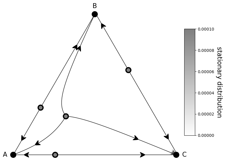
[22]:
fig, ax = plt.subplots(figsize=(10,8))

plot = (simplex.add_axis(ax=ax)
           .apply_simplex_boundaries_to_gradients(Ux, Uy)
           .draw_stationary_points(roots_xy, stability)
           .add_vertex_labels(type_labels)
           .draw_stationary_distribution(sd, vmax=0.0001, alpha=0.5, edgecolors='gray', cmap='binary', shading='gouraud')
           .draw_trajectory_from_roots(lambda u, t: Z*evolver.full_gradient_selection_without_mutation(u, beta),
                                       roots,
                                       stability,
                                       trajectory_length=30,
                                       linewidth=1,
                                       step=0.001,
                                       color='k', draw_arrow=True, arrowdirection='right', arrowsize=30, zorder=4, arrowstyle='fancy')
          )

ax.axis('off')
ax.set_aspect('equal')

plt.xlim((-.05,1.05))
plt.ylim((-.02, simplex.top_corner + 0.05))
plt.show()