Simplified 2-Simplex plot

In the Plot the evolutionary dynamics in a 2-Simplex example, we show how to use the Simplex2D class to visualize dynamics on a 2 Simplex using arbitrary gradient function (although the examples were shown only for the replicator equation and the Moran process defined in a finite population of strategies).

However, when we want to use the replicator_equation and StochDynamics provided in egttools, then we can simplify the plotting process by using two utility functions: egttools.plotting.plot_replicator_dynamics_in_simplex and egttools.plotting.plot_pairwise_comparison_rule_dynamics_in_simplex.

import numpy as np
import matplotlib.pyplot as plt

%matplotlib inline

from egttools.plotting.simplified import plot_replicator_dynamics_in_simplex, plot_pairwise_comparison_rule_dynamics_in_simplex_without_roots
from egttools.utils import calculate_stationary_distribution

Evolutionary dynamics in infinite populations

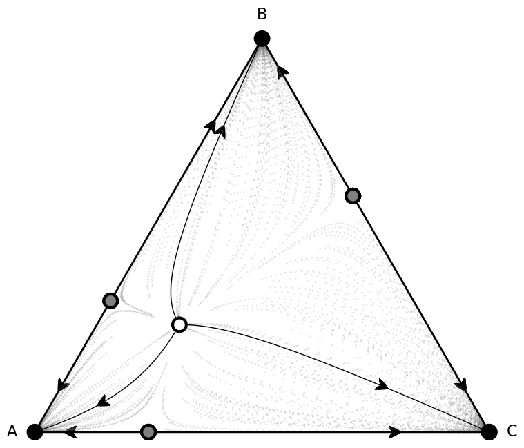
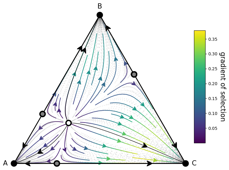
In infinite populations the dynamics are given by the replicator equation. Following we calculate the gradients for all the points in a grid and plot them in a 2-simplex using the Simplex2D class.

We will also be plotting in the simplex the stationary points. We will use black circle to represent stable equilibrium and white circles to represent unstable ones. The arrows indicate the direction of the selective pressure.

Define payoff matrix

payoffs = np.array([[1, 0, 0],
                    [0, 2, 0],
                    [0, 0, 3]])

type_labels = ['A', 'B', 'C']

Plot the trajectories from the stationary points

fig, ax = plt.subplots(figsize=(10,8))

simplex, gradient_function, roots, roots_xy, stability = plot_replicator_dynamics_in_simplex(payoffs,
                                                                                             nb_of_initial_points_for_root_search=100,
                                                                                             ax=ax)

plot = (simplex.draw_triangle()
           .add_vertex_labels(type_labels)
           .draw_stationary_points(roots_xy, stability)
           .draw_trajectory_from_roots(gradient_function,
                                       roots,
                                       stability,
                                       trajectory_length=15,
                                       linewidth=1,
                                       step=0.01,
                                       color='k', draw_arrow=True, arrowdirection='right', arrowsize=30, zorder=4, arrowstyle='fancy')
           .draw_scatter_shadow(gradient_function, 300, color='gray', marker='.', s=0.1)
          )

ax.axis('off')
ax.set_aspect('equal')

plt.xlim((-.05,1.05))
plt.ylim((-.02, simplex.top_corner + 0.05))
plt.show()

Plot the gradient field using a streamplot

fig, ax = plt.subplots(figsize=(10,8))

plot = (simplex.add_axis(ax=ax)
           .draw_triangle()
           .draw_gradients(zorder=0)
           .add_colorbar()
           .add_vertex_labels(type_labels)
           .draw_stationary_points(roots_xy, stability)
           .draw_trajectory_from_roots(gradient_function,
                                       roots,
                                       stability,
                                       trajectory_length=15,
                                       linewidth=1,
                                       step=0.01,
                                       color='k', draw_arrow=True, arrowdirection='right', arrowsize=30, zorder=4, arrowstyle='fancy')
           .draw_scatter_shadow(gradient_function, 300, color='gray', marker='.', s=0.1, zorder=0)
          )

ax.axis('off')
ax.set_aspect('equal')

plt.xlim((-.05,1.05))
plt.ylim((-.02, simplex.top_corner + 0.05))
plt.show()

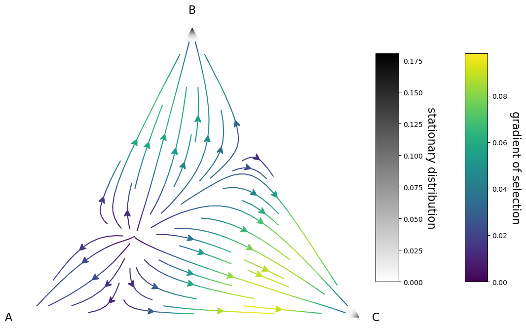
Stochastic Dynamics in finite populations - Moran process with pairwise comparison

In finite populations we will model the dynamics using a Moran process. The calculation of the gradients is implemented in EGTtools in the StochDynamics class. In this case, since we want to calculate the gradient at any point in the simplex, we will use the full_gradient_selection method

Define the population size and the intensity of selection

Z = 100
beta = 1
mu = 1/Z

Plot the gradient field and the stationary distribution

We can also plot the stationary distribution inside the simplex. It will give us an idea on where our population is going to spend most of the time

fig, ax = plt.subplots(figsize=(15,10))

simplex, gradient_function, game, evolver = plot_pairwise_comparison_rule_dynamics_in_simplex_without_roots(payoff_matrix=payoffs, population_size=Z, beta=beta, ax=ax)

transitions = evolver.calculate_transition_matrix(beta=beta, mu=mu)
sd = calculate_stationary_distribution(transitions.transpose())

plot = (simplex.add_axis(ax=ax)
           # .draw_triangle()
           .draw_gradients(zorder=5)
           .add_colorbar()
           .add_vertex_labels(type_labels)
           .draw_stationary_distribution(sd, alpha=1, edgecolors='gray', cmap='binary', shading='gouraud', zorder=0)
          )

ax.axis('off')
ax.set_aspect('equal')

plt.xlim((-.05,1.05))
plt.ylim((-.02, simplex.top_corner + 0.05))
plt.show()